Quickstart

In this tutorial, you will learn how you can set up a simple directed acyclic graph (DAG) to generate data from. For a more detailed description of DagSim’s workflow, see How to specify a simulation.

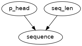
Suppose that we want to simulate sequences of coin tosses, based on a randomly generated probability of getting heads − per sequence − and random sequence length bounded between a low and a high value.

• \(sequence\_length \sim Cat(10,20)\), i.e. categorical distribution over integers between 10 and 20.

• \(p\_head \sim \mathcal{U}(0,1)\), i.e. standard uniform distribution

• \(sequence\): a sequence of coin tosses

We can do that using DagSim by following these steps:

Step 1: Setting up DagSim

To use DagSim for this tutorial, you can either install it on your machine by following the instructions on this page, or start a Binder session by clicking on the badge in one of the tabs below.

Step 2: Defining the simulation

Now, that we have DagSim set up, we want to specify and run the simulation. For that, we can use either python code or a YAML specification file. Regardless of the method you choose, you start by defining your own functions, if any, that will be used for the simulation.

Click on the corresponding tab for more details:

PythonYAML

We begin by importing the following:

import dagsim.base as ds
import numpy as np

1. Defining the functions:

The first thing that we need to define is the functions that relate the nodes to each other. For the model that we have defined above we would need three functions, one to sample data from a given Gaussian distribution, one that adds two numbers, and one that squares a number and adds a constant to it.

For \(p\_head\) and \(sequence\_length\) we can use the np.random.uniform and the np.random.randint functions, respectively, from numpy. For the sequence node, we would need to define our own function, e.g.:

from random import choices

def simulate_sequence(seq_len, p_head):
    return "".join(choices(["H", "T"], [p_head, 1-p_head], k=seq_len))

This functions would inform DagSim how to simulate the value of \(sequence\) based on the values of its parents.

2. Defining the graph:

Since \(p_\head\) uses the default arguments of the np.random.uniform function, we don’t provide any arguments for the function, only the name of the node and the function itself. For the nodes \(sequence\_length\) and \(sequence\), we need to give each node a name, the function to evaluate, and the arguments of the corresponding functions.

Passing these arguments mimics the way this is done in Python. These arguments can be either positional arguments (provided in the form of a list of the arguments’ values), keyword arguments (in the form of a dictionary with (arg_name:arg_value) keys-value pairs), or a combination of both. For more information on different ways to pass arguments, check this tutorial. In this example, they are all passed as positional arguments.

sequence_length = ds.Node(name="sequence_length", function=np.random.randint, args=[10, 20])
p_head = ds.Node(name="p_head", function=np.random.uniform)
sequence = ds.Node(name="sequence", function=simulate_sequence, args=[sequence_length, p_head])

At this stage, we can simply compile the graph as follows:

listNodes = [sequence_length, p_head, sequence]
my_graph = ds.Graph(listNodes, "Graph1")

Once we have compiled the graph, we can draw it to get a graphical representation of the underlying model, as follows:

my_graph.draw()

3. Running the simulation:

Now that we have defined everything we need, we simulate the data by calling the simulate method and providing the number of samples and the name of the CSV file to which to save the data.

data = my_graph.simulate(num_samples=100, csv_name="hello_world")