Simulate data for a simple linear regression problem

In this tutorial, you will learn how to build a simple DAG using DagSim to generate data for a simple linear regression problem, using either python code or a YAML configuration. If you are not familiar with the workflow of DagSim, see How to specify a simulation.

Define the simulation using python code

To run this tutorial on binder, click on this badge:

We begin by importing the following:

import dagsim.base as ds
import numpy as np
from sklearn.linear_model import LinearRegression as lr
import pandas as pd

1. Defining the functions:

The first thing that we need to define is the functions that relate the nodes to each other. In our example, we need one function for simulating the value of the feature \(x\) and another function to specify the true relation between \(x\) and the output \(y\).

For simplicity, we will simulate x to follow a standard normal distribution. For \(y\), suppose that the ground truth relation is: \(y = 2x + 1 + \epsilon\), where \(\epsilon\) is a white noise error term . Suppose that we also want to have control of the standard deviation of this error term from DagSim.

We can then define such a function in python as the following:

def ground_truth(x, std_dev):
  y = 2 * x + 1 + np.random.normal(0, std_dev)
  return y

This function would inform DagSim how to simulate the value \(y\) for each value of \(x\).

2. Defining the graph:

For the node of the variable \(x\) we only need to give it a name and the function to evaluate. This is because it has no parents, i.e. it is a root node, and the function to evaluate \(x\) does not need any arguments in our case. For the node of the variable \(y\), we need to give it a name, the function to evaluate, and the values of the arguments needed to evaluate that function, in the form of a dictionary, as shown below:

Nodex = ds.Node(name="x", function=np.random.normal)
Nodey = ds.Node(name="y", function=ground_truth, kwargs={"x": Nodex, "std_dev": 1})

At this stage, we can simply compile the graph as follows:

listNodes = [Nodex, Nodey]
my_graph = ds.Graph("Graph1", listNodes)

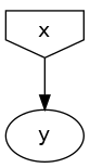
Once we have compiled the graph, we can draw it to get a graphical representation of the underlying model:

my_graph.draw()

3. Running the simulation:

Now that we have defined everything we need, we simulate the data by calling the simulate method and providing the number of samples and the name of the CSV file to which to save the data. We will run two simulations using the same model, one for training data and another for testing data.

train = my_graph.simulate(num_samples=70, csv_name="train")
test = my_graph.simulate(num_samples=30, csv_name="test")

4. Running the analysis:

Here, we will use the linear regression model by scikit-learn to run the analysis, and pandas to read the CSV files. Note that this step is not DagSim-specific and is up to the user to define the workflow of the analysis. We can use the dictionary returned by the simulate method, which contains the data, or read the saved CSV files. Here, we will use the second method.

First, we need to read the training dataset in order to train the model:

train_data = pd.read_csv("train.csv")
print(train_data.head())

x_train = train_data.iloc[:, 0].to_numpy().reshape([-1, 1])
print("x_train", x_train.shape)
y_train = train_data.iloc[:, 1].to_numpy().reshape([-1, 1])
print("y_train", y_train.shape)

After that we train a linear regression model as follows:

LR = lr()
reg = LR.fit(x_train, y_train)
reg.score(x_train, y_train)
print("Coefficient: ", LR.coef_)
print("Intercept: ", LR.intercept_)

Now, we evaluate the model by first reading the testing data set, and then calculating the \(R^2\) coefficient:

test_data = pd.read_csv("test.csv")
x_test = test_data.iloc[:, 0].to_numpy().reshape([-1, 1])
print("x_test", x_test.shape)
y_test = test_data.iloc[:, 1].to_numpy().reshape([-1, 1])
print("y_test", y_test.shape)
print("R2 score on test data: ", LR.score(x_test, y_test))